1 Executive Summary
We investigate the possibility of using Gaia observations as a source of calibration stars for LSST observations. A population of suitable Gaia stars could make it unnecessary to run ubercal on the LSST data. We find simulated Gaia BP/RP spectra can generate synthetic g, r, i, z, and y magnitudes for stars with adequate precision that they could be used to calibrate zeropoint magnitudes for individual LSST CCDs.
The Gaia specrta to not extend far enough into the blue to compute LSST u magnitudes. We explore the possibility of interpolating u magnitudes from Kurucz stellar models using the Gaia synthetic g and r magnitudes along with the Gaia fitted metallicity and surface gravity fitted values. We find the interpolating u magnitudes is very sensitive to the metallicity and would only be adequate with a larger stellar atmosphere library and/or better interpolation scheme.
One final warning is that in the galactic plane, Gaia will only observe brighter stars. Since the BP/RP observations only share about 2 magnitudes of overlap with LSST, this means Gaia will not provide usable calibration stars for any filter in the galactic plane.
2 Introduction
Running self-calibration (aka ubercal) on an LSST-sized dataset is difficult (though not impossible). It would be convenient if there was an external source of calibration stars we could use to set LSST observation zeropoints.
3 Gaia and ULYSSES
The Gaia mission will observe around a billion stars. The BP/RP spectrograph will take low resolution spectra of the Gaia targets. ULYSSES can simulate the expected BP/RP observations given a stellar spectrum as input.
Python wrappers to the ULYSSES code can be found in the sims_Gaia_calib repo.
4 Generating a Gaia-like Catalog
By default, ULYSSES output is in terms of electrons. To calibrate the output spectra to physical units, we run a flat spectrum source through ULYSSES and use the noiseless output to define the instrument response function. We are essentially assuming Gaia will be able to calibrate it’s spectra to a level where the calibration does not significantly contribute to the final spectra noise. With the calibrated ULYSSES spectra, we can compute synthetic LSST magnitudes for the g,r,i,z,y filters. The BP spectra do not extend far enough into the blue to compute LSST u magnitudes.
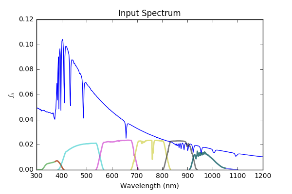
Figure 1 Example stellar spectrum input to ULSYSSES with the LSST filters shown. The LSST u-band is shaded brown where it has overlap with Gaia.
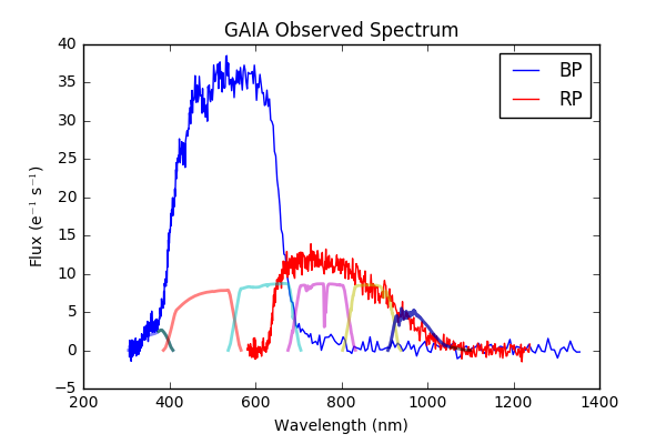
Figure 2 Example of the resulting BP/RP spectra when the input spectrum is passed through ULYSSES.
The BP and RP channels have a region of overlap. For simplicity, we use the BP output blueward of 675 nm and the RP output redward. In theory, one could slightly increase the SNR in the overlap region by properly weighting and combining the spectra. This would only impact the LSST r filter.
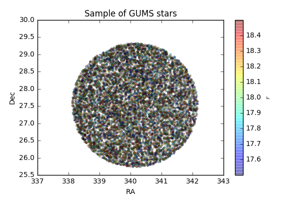
Figure 3 A limited magnitude range of the stars used.
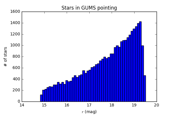
Figure 4 Histogram of the r-band stellar magnitudes used from GUMS and simulated with ULYSSES.
We use a subset of the Gaia GUMS catalog to generate Gaia end-of-mission (i.e., 75 transits) quality spectra for all the stars down to G~20 in a single LSST pointing. For each star, we assign a suitable Kurucz model SED and use ULYSSES to compute a Gaia specrtum. We then compute synthetic LSST magnitudes for each star.
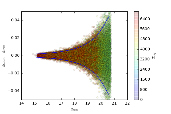
Figure 5 Residuals of recovered g magnitudes. Blue lines show the 2-sigma (robust) RMS envelope.
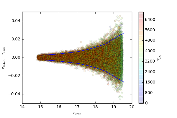
Figure 6 Residuals of recovered r magnitudes.
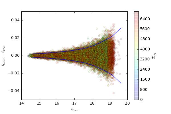
Figure 7 Residuals of recovered i magnitudes.
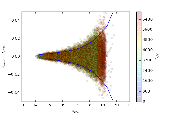
Figure 8 Residuals of recovered z magnitudes.
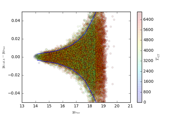
Figure 9 Residuals of recovered y magnitudes.
5 Results
Note the GUMS field which we used is located at (RA, dec) = (340.104, 27.547) aka (l,b)=(87.23, -25.0) with 33,000 stars (13,000 in the range 17 < g < 19). Scaling to the galactic pole, we would expect the density of stars to drop to ~25% that level. So we would still have ~30 Gaia stars per LSST CCD at the galactic pole that could be used for calibration.
We test how much area would be needed to calibrate a zeropoint to 5 millimag precision. In each filter, we use the magnitude range 17-18, and use our model of Mlky Way stellar density to scale the expected number of stars from our example GUMS location. For reference, a single LSST CCD is 176 sq arcmin in size. Thus, even at the galactic poles, we expect there should be enough Gaia stars measured with high enough precision to calibrate at the CCD scale (the y-band is starting to push the limit).
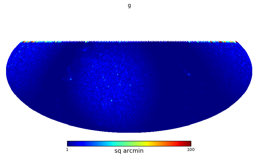
Figure 10 Area needed to calibrate zeropoint to 5 millimags.

Figure 11 Area needed to calibrate zeropoint to 5 millimags.
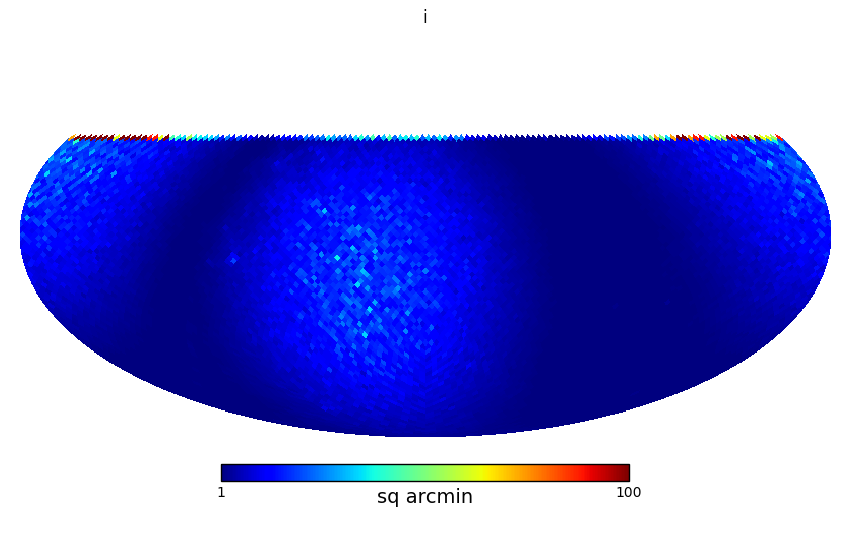
Figure 12 Area needed to calibrate zeropoint to 5 millimags.

Figure 13 Area needed to calibrate zeropoint to 5 millimags.
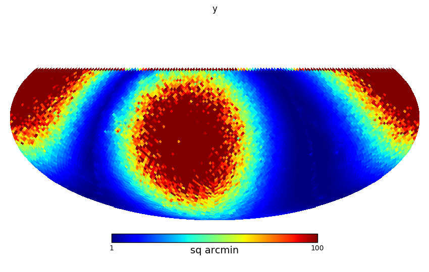
Figure 14 Area needed to calibrate zeropoint to 5 millimags.
6 Recovering the u-band
The synthetic y-band magnitudes are still usable because the LSST y throughput is very low in the region where Gaia cuts off. That is not true for the u-band, thus, if we are going to use Gaia to calibrate the u filter, there needs to be an extra step in extrapolating Gaia observations to LSST u-magnitudes.
One possible solution is to use Gaia derived stellar parameters (Teff, Fe/H, log g) along with Kurucz models to interpolate the expected LSST u magnitude. Lui et al look at how well Gaia will be able to recover stellar parameters.
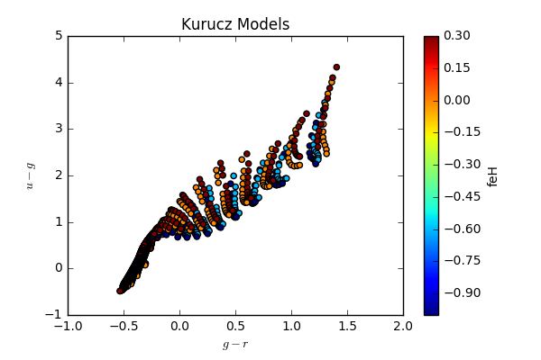
Figure 15 Kurucz model grid.
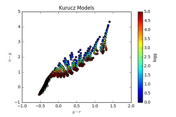
Figure 16 Same as Figure 15, but color-coded by stellar log g.
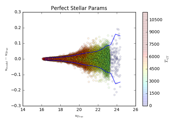
Figure 17 If we assume Gaia returns perfect stellar parameters, the Gaia synthetic LSST g and r magnitudes can be used with the Kurucz models to generate LSST u magnitudes with the plotted residual distribution. Results in 0.005 mag RMS at u=18, with the dispersion due to the errors in the g and r photometry.
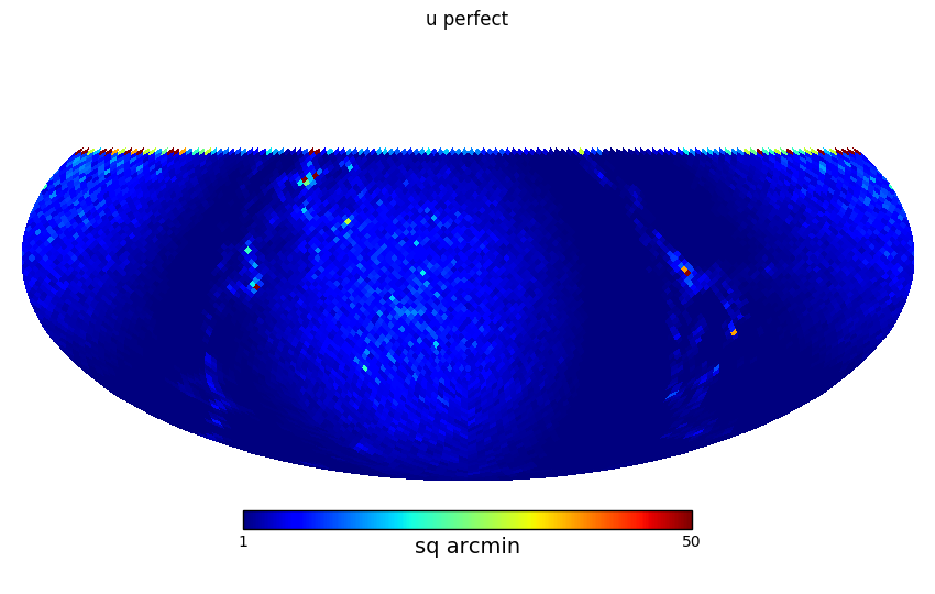
Figure 18 The area needed to calibrate the u-band to 0.01 mag zeropoint precision with perfect knowledge of stellar parameters.
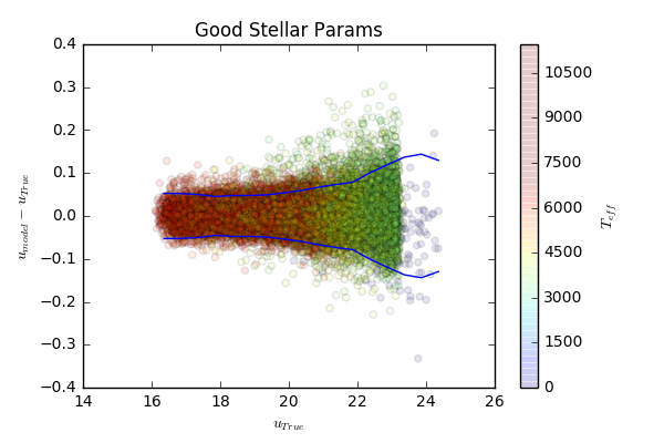
Figure 19 Same as Figure 17, but inserting 0.1 dex RMS errors in the metallicity and 0.2 dex in log g Gaia values. Results in 0.025 mag RMS at u=18.
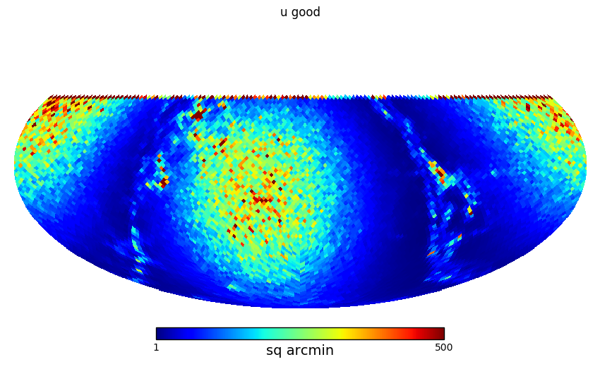
Figure 20 The area needed to calibrate the u-band to 0.01 mag zeropoint precision if the stellar parameters are “good”.
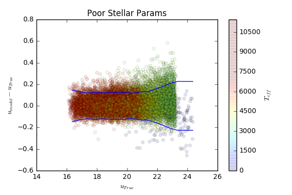
Figure 21 Same as Figure 17, but inserting 0.3 dex RMS errors on the metallicity and 0.5 dex errors on log g. Results in 0.065 mag RMS at u=18.
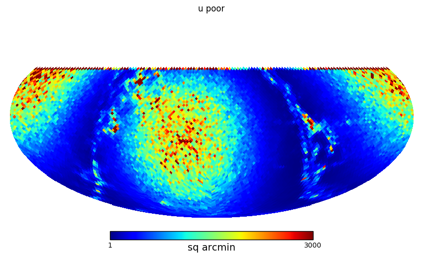
Figure 22 The area needed to calibrate the u-band to 0.01 mag zeropoint precision if the stellar parameters are “poor”.
It should be possible to construct a u-band stellar catalog from the Gaia data that would be adequate for calibrating LSST observations if
- stars can be described by Kurucz models
- Gaia returns stellar parameters with their expected precision
Here we check on how well Kurucz models can convert Gaia observations into u-g colors. We take the stsci grid of models (plotted in Figure 15) and withhold a random 10% of the points (110 points) and use the remaining 90% (990 points) to interpolate the expected u-g color using the scipy LinearNDInterpolator which uses Qhull and rescales the input dimensions. For red stars (u-g > 0.5), the u-g color of the interpolated points has an RMS error of 0.04 mag. It may be possible to reduce the interpolation error by using a finer grid of stellar atmospheres, or possibly using a more sophisticated interpolation method. The interpolation seems to be very sensitive to the stellar metalicity (e.g., it does a poor job interpolating of there are not similar metallicity points nearby).
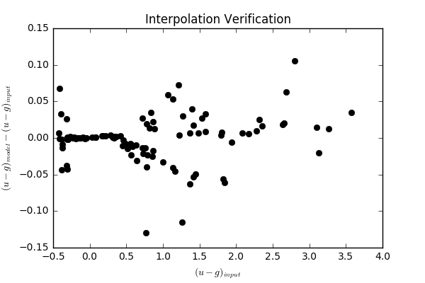
Figure 23 Testing the ability to correctly interpolate u-g color from Kurucz models given g-r, metallicity, and log g. No random errors were introduced.
7 Other Issues
Besides the difficulty in extrapolating the u-band, Gaia will not observe as deep in the galactic plane. This leaves the possibility that there will not be any overlap in the Gaia observations and LSST stars that are not saturated.
The Gaia data release scenarios do not include releasing the reduced BP/RP spectra, but only the derived stellar parameters. Thus we may need to request the Gaia collaboration compute synthetic LSST magnitudes or expand the scope of their data releases to include BP/RP (non-integrated) spectra.